Distributed Transitive Closure Algorithms, Part 2 – Seminaive and Smart

Seminaive

The seminaive algorithm is an example of a linear transitive closure algorithm. Initially, the transitive closure contains only the original edges from the graph. Then, at each round, the transitive closure is expanded by combining the pairs found so far with an additional edge from the base graph. In order to compute the transitive closure using the seminaive algorithm, the number of iterations required is equal to one less than the graph’s diameter (From Wikipedia: To find the diameter of a graph, first find the shortest path between each pair of vertices. The greatest length of any of these paths is the diameter of the graph). For an illustration of this, the figure below demonstrates the sequence of derivations produced by the seminaive algorithm in finding a pair of nodes connected by a path of length 4.

Seminaive: Rounds Required to Derive (a, e)

The pseudocode for the seminaive algorithm is presented below:

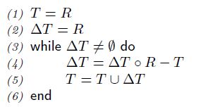
Seminaive Pseudocode

denotes the original graph. is initialized to , and will contain the transitive closure of upon termination. contains the newly derived tuples from the previous round. At each iteration of the while loop, is updated by joining with the edges of the original graph, .

On iteration , contains all pairs of nodes such that a shortest path between them has length . These pairs could not have been discovered in a previous round (by virtue of the shortest path between them having length ). If any pair produced by the join has already been found, then this implies there exists a shorter path between the two nodes which was found on a previous iteration. The set difference operation removes any such tuples. At the end of iteration , every tuple in represents a newly discovered tuple in the transitive closure.

The reasoning behind algorithm’s “seminaive” naming is that it avoids the fully naive join, which would perform the join at each iteration. This is enabled by exploiting the knowledge that the only new tuples possible from a join of at iteration come from elements of that were newly derived at iteration ; these newly derived tuples are exactly the contents of in seminaive.

Smart

Smart is an example of a nonlinear transitive closure algorithm. Instead of combining the current knowledge of the transitive closure with the edges of the base graph, each iteration of the smart algorithm combines (in a clever, or “smart”, way) the current transitive closure relation with itself. This enables the Smart algorithm to terminate in a number of rounds logarithmic in the graph’s diameter.

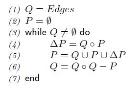
Smart Pseudocode

Smart iteratively builds two relations. At iteration , holds all pairs of nodes between which the length of the shortest path is exactly equal to . holds all pairs of nodes between which the shortest path has length less than .

In the first round of the computation, is simply a self-join of the original edges; in fact, all the transitive closure algorithms discussed here begin with this first step. The result of this join contains all pairs of nodes connected by a path of length 2, but there may be nodes in this result that are connected by a shorter path (a direct edge) so the set difference operation in line 6 is required to remove any pairs of nodes where there exists a path between them of length less than 2. In the next iteration, is again be joined with itself, producing (after the set difference) all pairs of nodes connected by a shortest path of exactly length 4.

In round , is formed from the join of and . This combines paths from (of length exactly ) with paths from (of length strictly less than ). This will find all shortest paths of any length between and . To also incorporate previously discovered paths of lesser length, line 5 takes the union of with the tuples of and . Therefore, at the end of round , contains all paths of length less than .

Not shown in the pseudocode is a duplicate elimination step after line 5, to remove redundant tuples produced by the join and union operations that form . Duplicate elimination is required on the relation for termination detection in the presence of cycles, and is implicit in the set difference operation of line 6. However, duplicate elimination on is not required to detect termination, but it is necessary for efficient performance on graphs where Smart will produce duplicate derivations.